
AIPE Field Simulation
AIPE Field Simulation is the finite-element agent in the AIPE framework. It drives the open-source tools Gmsh and Elmer to solve the thermal, magnetostatic and eddy-current problems of power-electronics design, and records every solve as an auditable case. This page explains the framework it belongs to, its role there, how the agent is organised, and the heat sink of a 10 kW DAB converter that it has solved.
The AIPE Framework
AIPE (AI for Power Engineering) is the open engineering ecosystem I am building through AIPE Labs. It treats power-converter design as a coordinated, iterative optimisation process rather than a chain of separate tools. Specialist agents each own one engineering step: electrical sizing, schematic drawing, circuit simulation, device and magnetics selection, thermal and field analysis, mechanical CAD and PCB layout. They exchange explicit inputs, assumptions, results and evidence through a shared Engineering State.
A workflow engine runs these steps as a checkpointed task graph. Results from later stages, such as magnetics or finite-element parameters, feed back into the circuit model, and every result is recorded against a verification gate. Software checks do not replace engineering review, measurement or hardware qualification, which remain separate gates. The first full benchmark is a 10 kW dual-active-bridge converter (800 V → 400 V, 100 kHz).
Role of the Field Simulation Agent
Field Simulation is the solver-backed check on the analytical estimates made earlier in the design. The magnetics and thermal stages size a transformer and a heat sink with fast analytical models; this agent solves the actual fields in those geometries and reports how far the estimates hold. In the 10 kW DAB workflow it computes the leakage inductance of the selected transformer window in 2-D and the temperature of the selected heat sink in 3-D, each at two mesh levels; the workflow then reconciles the circuit model with the magnetics and field results.
| Interface | Content |
|---|---|
| Inputs | Model parameters in SI units (geometry, materials, currents, film coefficients); optionally a STEP model with its metadata from the CAD Agent, or an operating point from the Engineering State |
| Outputs | A case directory per solve with mesh, solver input, logs and fields, a summary of results and checks, and evidence records with tool versions and SHA-256 hashes |
| Hand-off | AIPE-Workflows records the results under its field-simulation gate and reconciles them with the circuit model; engineering review follows |
Results are verified against closed-form solutions and mesh refinement, not against measurements. The agent interface defines these inputs, outputs and limits.
How the Agent Is Organised
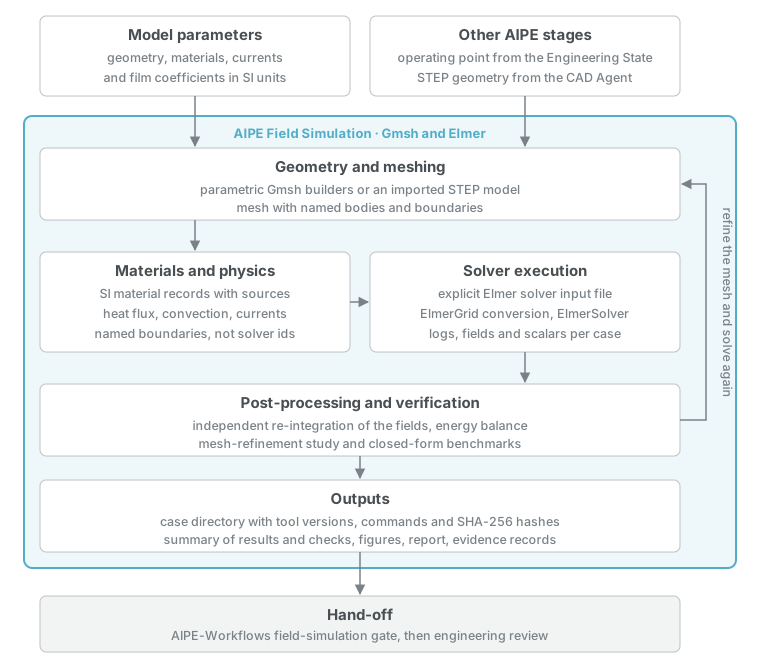
A simulation passes through five stages, and each stage hands the next a solver-neutral artefact, so only the solver-execution stage is specific to Elmer. Models and benchmarks are solved on successively finer meshes, so the discretisation error is measured rather than assumed.
| Part | Responsibility |
|---|---|
| Geometry and meshing | Parametric Gmsh builders, or an imported STEP model, produce a mesh whose bodies and boundaries carry named groups. |
| Materials and physics | SI material records with sources, and a problem description (heat flux, convection, adiabatic faces, currents) that refers to boundary names rather than solver identifiers. |
| Solver execution | Locates and qualifies Gmsh, ElmerGrid and ElmerSolver, renders an explicit solver input file and runs the case with logs. |
| Post-processing and verification | Re-integrates the solved fields independently with numpy, checks energy balance and compares refinement levels; four benchmarks compare against closed-form solutions. |
| Outputs | A case directory with tool versions, commands and SHA-256 hashes, a summary of results and checks, figures, a report and AIPE evidence records. |
Four benchmarks prove the chain before any design model is trusted: a conduction slab, a coaxial magnetostatic conductor, a 100 kHz copper skin-effect slab and a 3-D fin, each within a fraction of a percent of its analytical solution at the finest mesh. The architecture and benchmarks describe these stages in detail.
Example: Heat Sink for the 10 kW DAB Converter
This example solves the heat sink that the AIPE CAD Agent designed for one primary half-bridge of the AIPE benchmark converter: a 10 kW dual-active-bridge converter from 800 V to 400 V at 100 kHz. The agent reads the CAD Agent’s STEP model directly, so the geometry solved is the geometry that was designed. Two TO-247-4L SiC MOSFETs sit on alumina pads on a forced-air-cooled aluminium sink, and their losses, which rise with junction temperature, come from the AIPE Thermal Design loss model.
The example asks three questions: how hot the junctions get at the nominal operating point, how much margin remains to the 125 °C design target, and how strongly the answer depends on the cooling. One command runs the whole chain in about two minutes.
| Input | Value |
|---|---|
| Geometry | CAD Agent STEP model: 80 × 80 × 8 mm Al-6063 base (k = 209 W/m·K), 12 fins 1.5 mm thick and 35 mm tall at 5 mm pitch, 0.25 mm alumina pads (k = 24 W/m·K) |
| Devices | Two C3M0075120K-class SiC MOSFETs of one primary half-bridge, 9.67 A rms each, junction-to-case resistance 1.1 K/W |
| Loss model | Conduction loss with RDS(on) = 75 mΩ at 25 °C, rising to 1.7 times at 175 °C, plus 6.75 W turn-off loss: 13.76 W per device at 25 °C and 17.04 W at 125 °C |
| Cooling | Forced air, film coefficient 34.4 W/m²·K on the fin side, swept from 10 to 80 W/m²·K; 40 °C ambient |
| Limits | Junction design target 125 °C, maximum 175 °C |
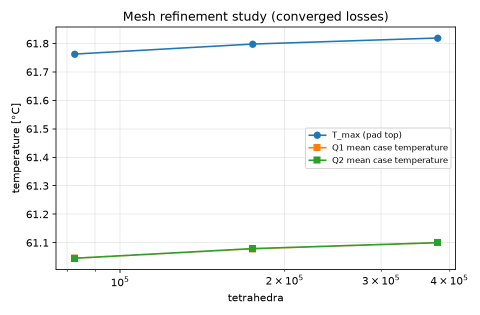
| Mesh | Three levels: 83,000, 175,000 and 380,000 tetrahedra |
From CAD Model to Mesh
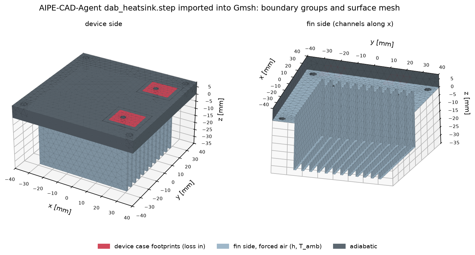
Gmsh imports the STEP model, identifies each solid by its CAD product name, and keeps the sink and both pads. It imprints each device tab footprint on its pad as the surface where the loss enters, drops the moulded bodies, leads, screws and bushings, and groups the faces into device cases, the forced-air fin side and the adiabatic remainder. The imported volumes and areas are checked against the metadata the CAD Agent recorded with the model.
Electrothermal Solution
The device loss depends on the junction temperature, which depends on the loss. With a fixed film coefficient, conduction in the sink is linear in the loss, and the loss is linear in the junction temperature, so the loop has a closed-form solution:
One finite-element solve per film coefficient gives the case-to-ambient resistance; the agent closes the loop and re-solves the model at the converged losses on all three meshes. At the nominal cooling, on the finest mesh, both devices settle at 15.50 W and a junction temperature of 78.2 °C, leaving 46.8 K of margin to the design target.
| At 34.4 W/m²·K, finest mesh | Q1 and Q2 |
|---|---|
| Loss, self-consistent with the junction temperature | 15.50 W |
| Case temperature, mean / maximum over the tab footprint | 61.10 / 61.82 °C |
| Junction temperature, case mean plus loss × Rth,jc | 78.2 °C |
| Margin to the 125 °C design target | 46.8 K |
| Case-to-ambient resistance, both devices heating | 1.361 K/W |
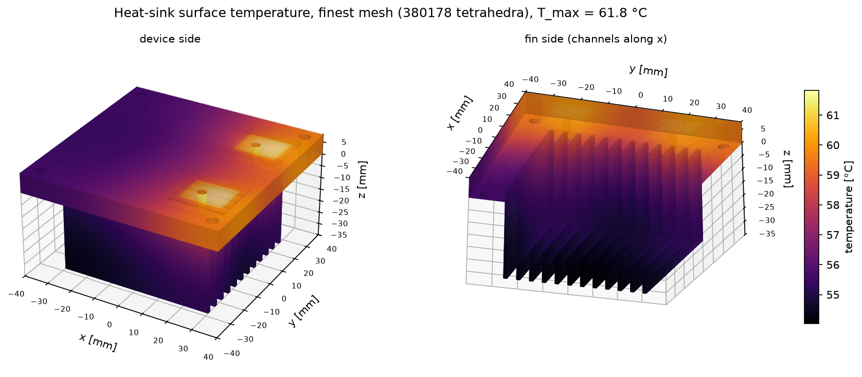
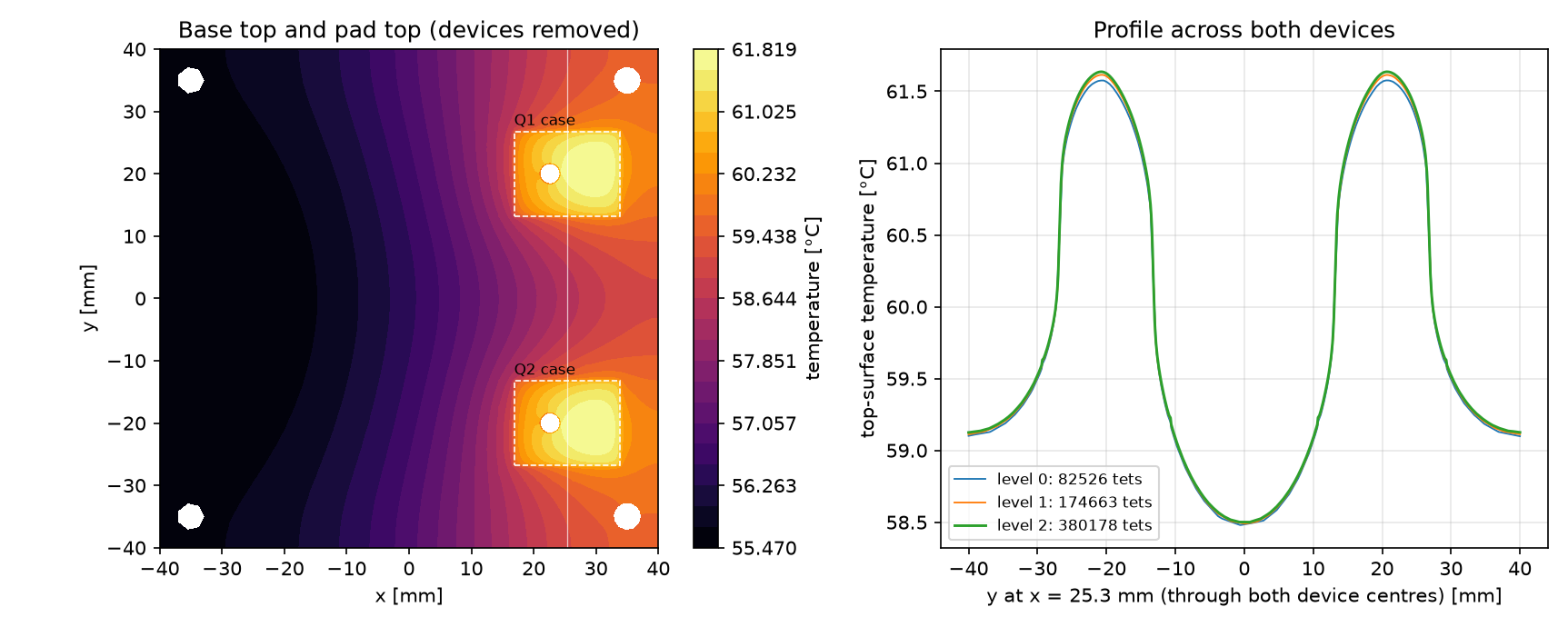
The top-surface map shows a design issue the analytical models cannot. The devices sit near the base edge, at x = 17 to 34 mm, while the fins span only x = −30 to +30 mm, so heat has to flow back across the base to reach the finned area.
Sensitivity to Cooling
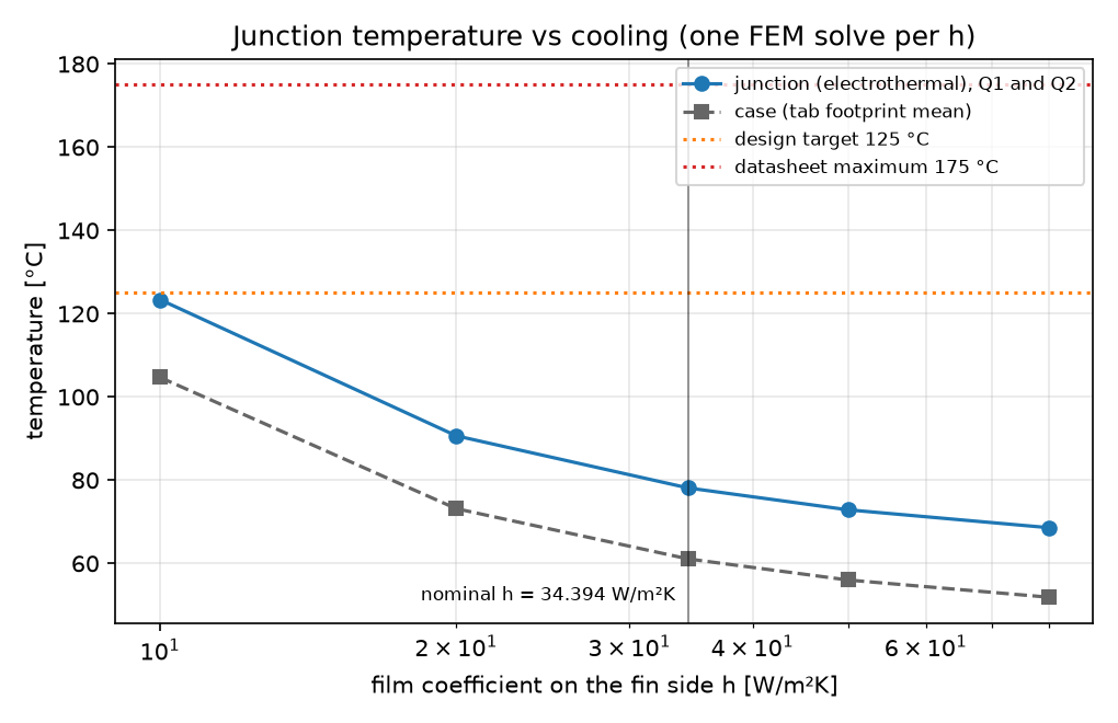
Sweeping the film coefficient shows that this sink depends on its fans. If the airflow collapses to 10 W/m²·K, which is typically still more than natural convection gives through 3.5 mm fin gaps, the junctions reach 123.4 °C, right at the design target. The sweep is solved on the middle mesh.
| Film coefficient (W/m²·K) | 10 | 20 | 34.4 | 50 | 80 |
|---|---|---|---|---|---|
| Junction temperature (°C) | 123.4 | 90.7 | 78.1 | 72.9 | 68.6 |
| Loss per device (W) | 16.98 | 15.91 | 15.50 | 15.33 | 15.19 |
Design Findings
Of the 38 K junction rise at nominal cooling, 17 K is the devices’ own junction-to-case resistance, which no sink can remove; 5.5 K is spreading through the pad and base; and 15.6 K is convection. Better airflow or more fin area therefore pays most, and a thicker base least. Moving the devices inboard, or extending the fins under them, is the next design iteration to hand back to the CAD Agent. For context only, the analytical forced-air model in AIPE Thermal Design, which uses different assumptions, converged at 71.1 °C.
Verification
| Check | Result |
|---|---|
| Energy balance: heat leaving the fin side equals the 31.0 W of losses | Error 6 × 10⁻¹¹ |
| Independent re-integration of the solved field matches the solver | Error 6 × 10⁻¹² |
| Imported solid volumes match the CAD Agent’s recorded volumes | Error 9 × 10⁻¹⁶ |
| Fin-side area matches the CAD Agent’s analytic area, less the through-holes | Error 6 × 10⁻¹⁶ |
| Two loss levels on one mesh give the same resistance, justifying the closed-form loop | Error 6 × 10⁻⁷ |
| The loss model at the final junction temperature reproduces the loss solved | Error 5 × 10⁻⁵ |
| The two mirror-symmetric devices see the same case temperature | 7 × 10⁻⁶ of the rise |
| Hotspot rise between the two finest meshes | Changes by 0.1% (limit 2%) |
Task Outputs
The task produced a case directory for each solve, with the mesh, solver input, logs and fields, together with a summary, figures and a report. The example runs on every push in continuous integration, and the published results come from such a run. The results are verified for internal consistency and discretisation error, not validated against measurements, and they carry the stated assumptions:
- the film coefficient is a uniform value on the fin side, taken from a correlation for a similar sink, without airflow simulation, radiation or air heating along the channels;
- each loss enters as a uniform flux on the tab footprint, without a die or package model, and contacts are ideal, so the case temperature is optimistic by roughly the loss × 0.05 K/W;
- the base top, edges and holes are adiabatic and heat through the leads is ignored, both conservative;
- the turn-off loss and the temperature factor of RDS(on) are assumptions of the loss model, to be replaced by device-database values.